Hello Dear Nektar forum, hope my message finds everyone well.
I have been working on a film-cooling hole nektar++ set-up case. I mainly followed the guidelines from Imperial front wing study and the user guide. I’ve run into a puzzling Taylor-Hood pressure issue that I’d appreciate some insight on.
Case set-u p
I started with a coarse linear mesh, has 200K nodes and 1million DOF at P=1. This mesh has one macro prism layer and uses NekMesh prism layer splitting to create the prism layers .
Channel U∞ = 10 m/s, with coolant supplied from a plenum at 0.1309 m/s to match a 10 m/s jet velocity at the hole. The geometry has two sharp features that make meshing difficult; since the bottom corner also has high gradients, I added a fillet there to avoid solver instabilities from skewed cel ls.
I use a RANS field to initialise start-up and start the solution from P=1. This calculation continued for 10 through-flows based on channel length (60D/Uinf; where D=0.00775 m and Uinf=10ms), just to make sure I have a stable starting point when increasing the polynomial order. (P= 1, CFL= 0.04, for testing purposes)
The issue
I then used part of the IFW condition xml file as a template to increase the polynomial order to P=2(NUMMODES=3) for velocity and leave the polynomial order at P=1(NUMMODES=2) for pressure, using a Taylor-Hood polynomial expansion. I tested 2 different variants of this.
Explicit form: (as shown in the my example following IFW below)
<EXPANSIONS>
<!-- C[0] = Prism C[1] = Tetra -->

<E COMPOSITE="C[0]" BASISTYPE="Modified_A,Modified_A,Modified_B" NUMMODES="3,3,3" POINTSTYPE="GaussLobattoLegendre,GaussLobattoLegendre,GaussRadauMAlpha1Beta0" NUMPOINTS="5,5,4" FIELDS="u,v,w" />

<E COMPOSITE="C[1]" BASISTYPE="Modified_A,Modified_B,Modified_C" NUMMODES="3,3,3" POINTSTYPE="GaussLobattoLegendre,GaussRadauMAlpha1Beta0,GaussRadauMAlpha2Beta0" NUMPOINTS="5,4,4" FIELDS="u,v,w" />

<E COMPOSITE="C[0]" BASISTYPE="Modified_A,Modified_A,Modified_B" NUMMODES="2,2,2" POINTSTYPE="GaussLobattoLegendre,GaussLobattoLegendre,GaussRadauMAlpha1Beta0" NUMPOINTS="5,5,4" FIELDS="p" />

<E COMPOSITE="C[1]" BASISTYPE="Modified_A,Modified_B,Modified_C" NUMMODES="2,2,2" POINTSTYPE="GaussLobattoLegendre,GaussRadauMAlpha1Beta0,GaussRadauMAlpha2Beta0" NUMPOINTS="5,4,4" FIELDS="p" />

</EXPANSIONS>
Secondly, I tested a compact form following the user guide as below;
    <E COMPOSITE="C[0,1]" NUMMODES="3" TYPE="MODIFIED" FIELDS="u,v,w" />
    <E COMPOSITE="C[0,1]" NUMMODES="2" TYPE="MODIFIEDQUADPLUS1" FIELDS="p" />
I attached the full version of my condition xml file.
The solver can run with a stable CFL throughout the calculation. However unfortunately, I cannot obtain a meaningful pressure field (unphysical values) although the velocity field is showing correct time evolution.
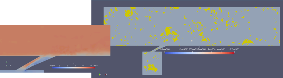
dt=10-7, CFL=0.04 (for testing purposes)
Example log output:
Writing: “cad3p_p12_dt107_6599.chk” (0.105439s, XML)
CPU time for filter Checkpoint: 0.106312s
Percentage of time integration: 44.765 %
Total filters CPU Time: 0.10631 2s
CG iterations made = 13 using tolerance of 1e-09 (error = 3.52241e-10, rhs_mag = 65.06 82)
CG iterations made = 51 using tolerance of 1e-09 (error = 9.66572e-10, rhs_mag = 2.40845e +08)
CG iterations made = 45 using tolerance of 1e-09 (error = 9.95594e-10, rhs_mag = 2.28485 e+08)
CG iterations made = 49 using tolerance of 1e-09 (error = 9.5522e-10, rhs_mag = 2.1676 1e+08)
Steps: 65995 Time: 0.0065995 CPU Time: 0. 230819s
CFL: 0.0412955 (in elm t 77680)
CG iterations made = 13 using tolerance of 1e-09 (error = 3.52414e-10, rhs_mag = 65.0671)
CG iterations made = 51 using tolerance of 1e-09 (error = 9.66698e-10, rhs_mag = 2. 40845e+08)
CG iterations made = 45 using tolerance of 1e-09 (error = 9.9577e-10, rhs_mag = 2 .28485e+08)
CG iterations made = 49 using tolerance of 1e-09 (error = 9.54988e-10, rhs_mag = 2.16761e+08)
Steps: 65997 Time: 0.0065997 CPU Ti me: 0.233592s
In the case I don’t use Taylor Hood Approximation and set the polynomial order to P=2 for both velocity and pressure, I am able to capture the accurate evolution for both velocity and pressure fields. (P= 2, dt=10-7, CFL= 0.04)
Another detail is the DOF calculated using FieldConvert utility, which is 3million for both cases that using Taylor-Hood appx. and P=2 for both pressure and velocity. Since the pressure polynomial order is lower with Taylor-Hood appx., I would have expected the total DOF to be lower accordingly.
I had several tests to overcome the issue such as initialising pressure to 0 at the start-up(s), testing different tolerances for pressure iterative solver or testing Taylor Hood appx with simplified case; a channel flow domain where the jet is defined as a BC at the wall to isolate the effect of the mesh difficulties, however these also resulted s imilarly.
- I would be very happy to have a bit more understanding of the Taylor-Hood approximation, and how I should be calculating number of points for different element types in case there are any mistakes in my de finitions.
- Are there any specific pressure boundary conditions should I be using at the walls for this f ormulation?
- I was also wondering whether the pressure is obtained through an iterative corrector loop within each timestep (as in PISO-type schemes) or reconstructed directly from the predicted velocity field via a single Poisson solve per step (fractional-step) to get a better understanding on velocity pressure coupling and how sensitive that reconstruction is to initialising pressure to 0 at start-up.
Any pointers or advice would be highly appreciated and thank you very much for your times and kind support.
Summary
This text will be hidden
<E COMPOSITE="C[0]" BASISTYPE="Modified_A,Modified_A,Modified_B" NUMMODES="3,3,3" POINTSTYPE="GaussLobattoLegendre,GaussLobattoLegendre,GaussRadauMAlpha1Beta0" NUMPOINTS="5,5,4" FIELDS="u,v,w" />

<E COMPOSITE="C[1]" BASISTYPE="Modified_A,Modified_B,Modified_C" NUMMODES="3,3,3" POINTSTYPE="GaussLobattoLegendre,GaussRadauMAlpha1Beta0,GaussRadauMAlpha2Beta0" NUMPOINTS="5,4,4" FIELDS="u,v,w" />

<E COMPOSITE="C[0]" BASISTYPE="Modified_A,Modified_A,Modified_B" NUMMODES="2,2,2" POINTSTYPE="GaussLobattoLegendre,GaussLobattoLegendre,GaussRadauMAlpha1Beta0" NUMPOINTS="5,5,4" FIELDS="p" />

<E COMPOSITE="C[1]" BASISTYPE="Modified_A,Modified_B,Modified_C" NUMMODES="2,2,2" POINTSTYPE="GaussLobattoLegendre,GaussRadauMAlpha1Beta0,GaussRadauMAlpha2Beta0" NUMPOINTS="5,4,4" FIELDS="p" />

</EXPANSIONS>

<CONDITIONS>

    <SOLVERINFO>
        <I PROPERTY="SolverType"                 VALUE="VelocityCorrectionScheme" />
        <I PROPERTY="EqType"                     VALUE="UnsteadyNavierStokes" />
        <I PROPERTY="AdvectionForm"              VALUE="Convective" />
        <I PROPERTY="Projection"                 VALUE="Galerkin" />
        <I PROPERTY="SpectralVanishingViscosity" VALUE="True" />
        <I PROPERTY="SPECTRALHPDEALIASING"       VALUE="True" />
    </SOLVERINFO>

    <GLOBALSYSSOLNINFO>

        <V VAR="u,v,w">
            <I PROPERTY="GlobalSysSoln"            VALUE="IterativeStaticCond" />
            <I PROPERTY="Preconditioner"           VALUE="LowEnergyBlock" />
        <!--    <I PROPERTY="IterativeSolverTolerance" VALUE="1e-9" />
            <I PROPERTY="NekLinSysMaxIterations"   VALUE="20000" /> -->
        </V>
        <V VAR="p">
            <I PROPERTY="GlobalSysSoln"            VALUE="IterativeStaticCond" />
            <I PROPERTY="Preconditioner"           VALUE="FullLinearSpaceWithLowEnergyBlock" />
        <!--    <I PROPERTY="IterativeSolverTolerance" VALUE="1e-9" />
            <I PROPERTY="NekLinSysMaxIterations"   VALUE="20000" /> -->
        </V>
    </GLOBALSYSSOLNINFO>

    <TIMEINTEGRATIONSCHEME>
        <METHOD> IMEX </METHOD>
        <ORDER> 1 </ORDER>
    </TIMEINTEGRATIONSCHEME>

    <PARAMETERS>
        <P> TimeStep        = 0.0000001   </P>
        <P> NumSteps        = 150000       </P>
        <P> IO_InfoSteps    = 1      </P>
        <P> IO_CFLSteps     = 1        </P>
        <P> Re              = 5100       </P>
        <P> Kinvis          = 0.0000149  </P>
        <P> SVVCutoffRatio = 0.3 </P>
        <P> SVVDiffCoeff   = 1.0 </P>
    </PARAMETERS>

    <VARIABLES>
        <V ID="0"> u </V>
        <V ID="1"> v </V>
        <V ID="2"> w </V>
        <V ID="3"> p </V>
    </VARIABLES>

    <BOUNDARYREGIONS>
        <B ID="0"> C[11] </B>           <!-- coolant inlet -->
        <B ID="1"> C[3]  </B>           <!-- main inlet -->
        <B ID="2"> C[5]  </B>           <!-- main outlet -->
        <B ID="3"> C[7]  </B>           <!-- periodic1 -->
        <B ID="5"> C[9]  </B>           <!-- periodic2 -->
        <B ID="7"> C[2,12,14,15] </B>   <!-- walls -->
    </BOUNDARYREGIONS>

    <BOUNDARYCONDITIONS>
        <REGION REF="0">    <!-- coolant inlet: T_c = 196 K -->
            <D VAR="u" VALUE="0" />
            <D VAR="v" VALUE="0" />
            <D VAR="w" VALUE="0.1309" />
            <N VAR="p" VALUE="0" />
        </REGION>
        <REGION REF="1">    <!-- main inlet: T_inf = 295 K -->
            <D VAR="u" VALUE="10" />
            <D VAR="v" VALUE="0" />
            <D VAR="w" VALUE="0" />
            <N VAR="p" VALUE="0" />
        </REGION>
        <REGION REF="2">    <!-- main outlet -->
            <N VAR="u" VALUE="0" />
            <N VAR="v" VALUE="0" />
            <N VAR="w" VALUE="0" />
            <D VAR="p" VALUE="0" />
        </REGION>
        <REGION REF="3">    <!-- periodic1 -->
            <P VAR="u" VALUE="[5]" />
            <P VAR="v" VALUE="[5]" />
            <P VAR="w" VALUE="[5]" />
            <P VAR="p" VALUE="[5]" />
        </REGION>
        <REGION REF="5">    <!-- periodic2 -->
            <P VAR="u" VALUE="[3]" />
            <P VAR="v" VALUE="[3]" />
            <P VAR="w" VALUE="[3]" />
            <P VAR="p" VALUE="[3]" />
        </REGION>
        <REGION REF="7">    <!-- adiabatic walls: no-slip, zero flux -->
            <D VAR="u" VALUE="0" />
            <D VAR="v" VALUE="0" />
            <D VAR="w" VALUE="0" />
            <N VAR="p" VALUE="0" />
        </REGION>
    </BOUNDARYCONDITIONS>

    <FUNCTION NAME="InitialConditions">
        <F VAR="u,v,w,p" FILE="cad3p_dt3_106_2_77.chk" />
            </FUNCTION>
</CONDITIONS>

<FILTERS>
    <FILTER TYPE="Checkpoint">
        <PARAM NAME="OutputFile">cad3p_p12_dt107</PARAM>
        <PARAM NAME="OutputFrequency">10</PARAM>
    </FILTER>
</FILTERS>