Downstream decay of turbulence in a flat-plate boundary layer using SEM + SPM trip at P2

[yaso]

Dear Nektar++ forum,

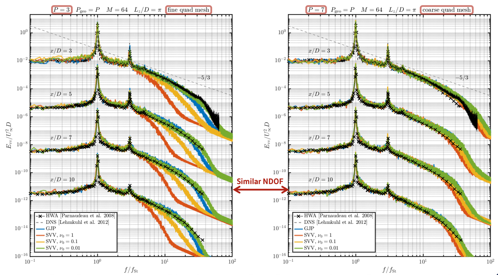
I am trying to reproduce the experimental turbulent boundary and have been encountering some issues with Synthetic Turbulence decaying downstream. I was wondering if anyone attempted to use this for a different case to the paper Isler et al. (2025) and would really appreciate any advice for the correct implementations.

I am using a structured mesh for this and I impose a mean turbulent boundary-layer velocity profile at the inlet fitted directly to the experimental data, and I use SEM to introduce turbulent fluctuations with the aim of sustaining this boundary layer as it develops downstream.

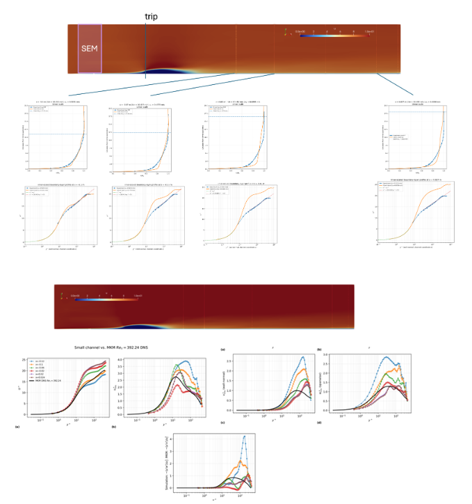
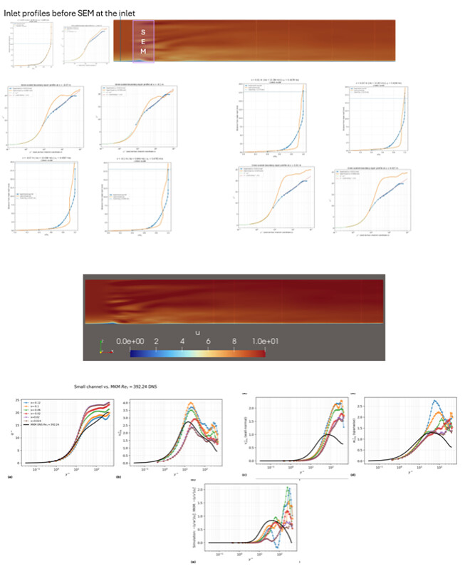
Although the inlet mean profile is already representative of the experimental turbulent boundary layer, the turbulence decays progressively downstream and mean velocity profiles move away from desired profile and becomes more laminar.

Another interesting detail is, when I plot the re stresses downstream of the trip or SEM, I observe a partial convergence towards the DNS Reynolds stresses (varies with uu,vv,ww) I used for SEM implementation, however mean boundary layer profile drifts from the turbulent state.

I have tested synthetic turbulence, an immersed-boundary trip using the Smoothed Profile Method (SPM) and both together. The combined SEM + SPM approach gives the closest agreement with the experimental mean velocity profile initially, but the fluctuations still decay further downstream and I have not yet obtained a sustained turbulent boundary layer over the required development length.

Current setup details:

• Incompressible Velocity Correction Scheme with SPM → Trip
• Incompressible Velocity Correction Scheme-> SEM
• P=2 (NUMMODES=3)
• IMEX, order 2
• Time step = 1x10^-5 s
• U_inf=10 m/s
• nu=1.49x10^-5 m²/s
• No-slip lower wall
• Free-slip upper boundary
• Spanwise-periodic boundaries
• Channel height = 38.75 mm
• Span = 46.5 mm
• Length= 261 mm
• Trip-wire radius = 3 mm, with its centre 1 mm below the wall, giving a 2 mm exposed height, has 2 spanwise wavelengths to break the symmetry across the span
• SPM smoothing thickness = 0.25 mm
• Spectral vanishing viscosity: DGKernel
• Spectral/hp dealiasing enabled

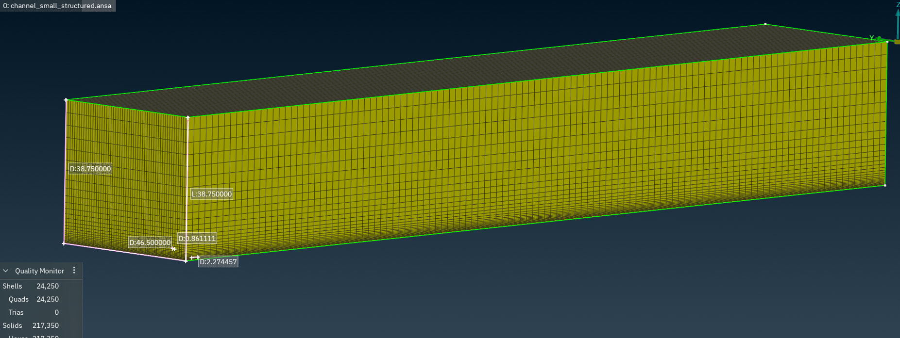
DOF= 5.8M @P2

My wall resolution for these cases resulted u_tau ~ 0.5 m/s, and appx. wall-unit resolution, note x, y and z are streamwise, spanwise and wall-normal resp.:

wall resolution
Streamwise spacing, x+	30
Spanwise spacing, y+	10
First wall-normal point, z+	0.458

These wall units are based on wall-averaged quantities / time-averaged over approximately two through flows based on domain length.

Synthetic turbulence strategy

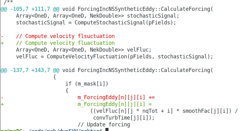
I have used Isler et al. (2025) as a reference for the source-term-based synthetic turbulence implementation and mainly followed the channel validation example. Below is a short summary of the Re stresses I used for SEM implementation.

Tests:

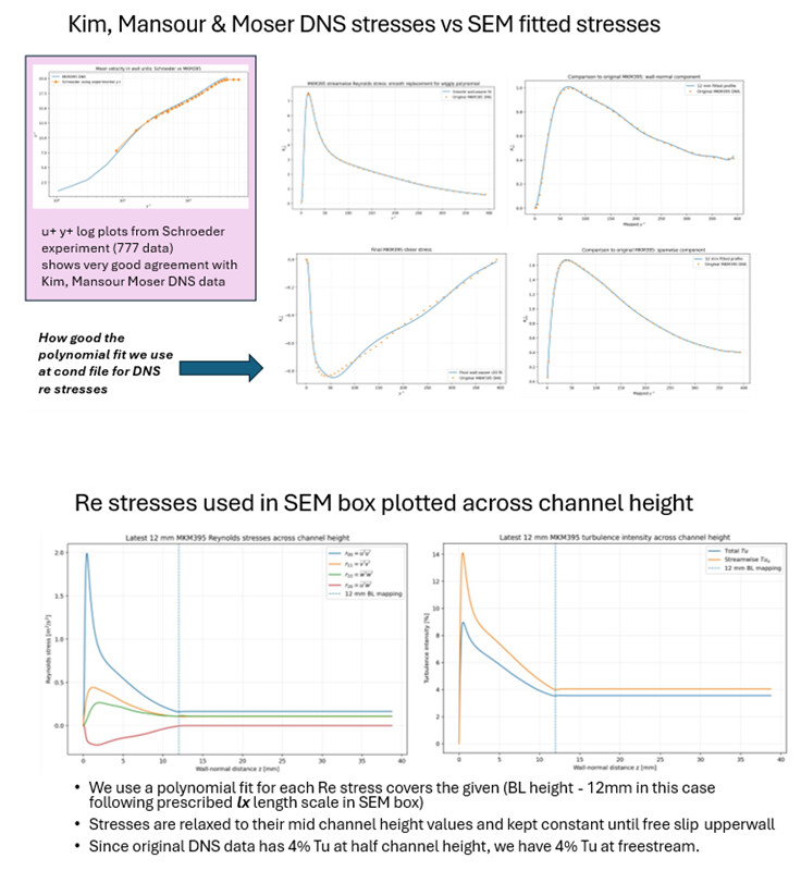
A. Reynolds stresses: I have tested profiles based on the Moser, Kim and Mansour Re_tau=395 channel DNS, mapped to the experimental boundary-layer thickness and to my coordinate system (Fig2). I have also tested simpler diagonal/isotropic stress tensors and profiles that approach prescribed free-stream turbulence levels.

B. Length scales: I have tested several anisotropic characteristic length-scale combinations. I mainly used 1.2x turbulent boundary layer height(following the paper again Isler et al. (2025)) and slightly increased in one case, the streamwise characteristic scale as 1.5 TBL height. Increasing or decreasing these scales has not clearly improved the downstream persistence of the turbulence.

Example 1.2 TBL height length scale scaling:

C. Turbulence intensity: I have varied the imposed turbulence intensity and the outer stress levels but have not observed a clear improvement in the downstream decay.

**Example provided Re stresses (Case3 below)
**
(plots available from link at the end of post link)

SEM + SPM gives the best agreement with the experimental mean profile. However, neither approach has yet produced turbulent fluctuations that remain sustained over the required downstream distance.

Mid-span time-averaged boundary layer profiles (linear &log) & Reynold Stresses:

Case1-Trip case with IBM + SEM:

Case3-SEM only using Kim, Moser Mansour DNS Channel data:

I suspected damping might effect the turbulence state downstream. There appears to be a strong sensitivity to spectral vanishing viscosity values, where even a tiny reduction in SVV parameters (currently using DG Kernel) makes the calculations diverge and SVV is not used in the above paper Isler et al. (2025).

I thought about implicit velocity correction scheme to maybe allow a larger CFL decreasing SVV but using this is not compatible with the SPM implementation (case3 where I got the closest profile to experiment). I had some trouble with my previous attempts to use this scheme for the type of cases with instantaneous divergence behaviour, which resulted in running but frozen flow fields. I am able to progressively decrease SVV for other set-ups (777 film cooling case) so I wondered whether there is a way to reduce in a stable way.

To my understanding I should be able to use only SEM and able to generate enough turbulence, so I would be very happy to have any suggestions what would be the most important checks.

My main points/questions are:

1. My wall resolution mainly matches with the Isler et al. (2025)
2. Is there a recommended diagnostic in Nektar++ for determining whether DGKernel SVV is removing a significant fraction of the turbulent fluctuations?
3. From the Isler et al. (2025) 5 delta(channel half height) should give a positive trend for converging the required boundary layer profile but maybe more development length is required? I have extracted profiles from 1-15 delta downstream.

I included more detailed information alongside some example xml condition files I have been using below hopefully would also be useful for people would like to use the method.

Synthetic Eddy Method Implementation tests using Nektar++.pptx

Any general recommendations to understand the root cause of the lack of turbulence downstream would be very valuable.

Thank you very much for your help!

[alexander.schukmann]

From my experience, given your comparatively low expansion order (P = 2), I would expect the DG-SVV kernel with the default value for the diffusion coefficient SVVDiffCoeff = 1 to introduce an excessive amount of dissipation, leading to the damping of the turbulence fluctuations you’re observing. For a given resolution, Gradient Jump Penalisation introduces less numerical dissipation but might require a reduced timestep. Similarly, reducing SVVDiffCoeff might require a timestep reduction to maintain stability at a given spatial resolution.
Alternatively, you could stick with the default value of the DG-SVV diffusion coefficient and increase the expansion order while coarsening the mesh skeleton accordingly to maintain approximately the same total number of DoFs. However, of course care should be taken to preserve sufficient near-wall resolution when redistributing the spatial resolution from h to p. This should shift the added dissipation towards the smallest resolved scales, which might have less of an impact on your Reynolds stresses.
I conducted a small study of flow around a cylinder a few years ago. The attached screenshot illustrates the aforementioned effects quite nicely for the spectra in the turbulent wake. I remember coming across a Nektar++ study that demonstrated this, but unfortunately I cannot find it at the moment. Maybe @ssherw knows which study I am referring to. In the paper by Moura et al., in which the GJP regularization was introduced in Nektar++, no variation of the SVV diffusion coefficient was performed, if I remember correctly.

[yaso]

Dear Alexander,

Thank you very much for your reply, the plot and papers - all of this information is very helpful.

SVV has been my strongest suspicion, but I had some trouble reducing it. In set-up case 3, where I use only SEM to sustain the turbulent boundary layer, reducing the timestep by a factor of 10 helped reducing the SVV and I will update the post with the results.

Another detail that may be useful for other users: Kim, Castro & Xie (2013, Comput. Fluids 84, 56–68) report that inserting synthetic turbulence too close to the inlet boundary in an incompressible solver creates larger spurious pressure fluctuations and recommend placing it at least ~0.5δ downstream. Isler et al. in their channel validation (2025, Int. J. Turbomach. Propuls. Power 10(3), 13, https://doi.org/10.3390/ijtpp10030013) place the centre of the synthetic eddy region at x/δ = 2 also. I ran another trip-wire case without SEM and it responds better to reducing the SVV in terms of stability. In my previous trip + SEM set-up the SEM box was closer to the inlet than this, so although I cannot fully confirm it, I suspect this might have made it difficult to reduce the SVV.

In the trip-only case, halving the SVV has not yet produced sustained turbulence yet but I continue testing with both methods and will update the post.

Thank you very much for your input, time and help again.

[mgao]

Hi yaso,

Thanks for the questions.

1. There is a bug in SEM of IncNS solver, which I have not reported to upstream yet. For now, it seems that bug will lead to a deviation of downstream profiles from reference. You may try it by your self (attached). We have a student just started to play with the SEM, and if have more info, will let you know.
   
   
2. It is found that source-type SEM requires quite a long time to recover physical turbulence, comparing with a normally-seen BC-type SEM, do check time convergence (e.g. energy) before doing analysis.
3. Since a trip itself can be used as a turbulence generation approach, test SEM and the trip separately can be more helpful.
4. As Alexander reported, try use SVV with a higher polynomial degree (e.g. P5-P7). This is the easiest way to get a good balance among robustness, efficiency and accuracy. If you have any stability issues with a higher polynomial degree, do let us know.